Wednesday, January 31, 2018

Trip to the 21st(?) Century

Went to Reading University last week, to do a lecture as part of a course for PhD students. The course was aimed at teaching paleodata students about models and how they might be useful for their research. A very good idea! Here are some students, and Joy (at the end of the bench) who was in charge, doing a lot of the teaching and most of the lecturing (a lot of work!) all while living up to her name!


Luckily, frothy coffee (a necessity for this travelling lecturer!) is as plentiful outside of Yorkshire as it  is inside. 


The main feature of Reading University campus is the pond which, at this time of year, is chock full of birds. I managed a couple of trips to inspect it, but I only had my iPhone so no point posting the bird pics. Here instead is some pond and trees.

Railway Britain does not seem to have advanced much since the 1980 and 1990s. Biggest difference is that the announcements at the stations are now audible. People also look at phones a lot more, and thankfully they shout into them a lot less. There are also places on the trains to plug your phone in to charge up its failing battery. 

Birmingham New Street station. Dangerously narrow platforms, with crowds standing well over the yellow line! ("Abunai desu kara kiiroi sen made osagari kudasai" - standard train announcement at all Japanese railway stations - because it is dangerous, stay back from the yellow line)


Reading station, however, was redeveloped THIS CENTURY! It's a sort of curvier, blue, dirty version of a late 20th century Japanese station. But at least it has nice wide platforms.


Settle-Reading is about 240 miles, taking about five and a half hours. I suppose this is an improvement over the seemingly endless period in the mid-1990s when all journeys took at least 10 hours due to every inch of track having to be inspected with a fine tooth comb. But it seemed like a lot of travelling for my 1.5 days in Reading. Trains back to the safety of the 19th century are rare and there was a long wait on an empty platform at Leeds station on Friday, but one can gain a little encouragement from the flavour of Victoriana emerging on the painted pillars.


Eventually... Ahhh, Settle station - back in the 19th century at last!


Monday, January 29, 2018

BlueSkiesResearch.org.uk: Cox et al part 3

As promised some more on this. The first thing I thought, on seeing this paper – a feeling that others apparently shared – was, why had no-one else already thought of this? Had we all just behaved like the fabled economist who, when their companion points out a £10 note lying on the pavement, ignores it, saying "If there really was a £10 note, someone would have picked it up already"?

Certainly the Schwartz fiasco will have put people off from pursuing this approach, as many of us had shown via a variety of arguments that the theoretical relationship in the simple 1-box climate model that directly links the autocorrelation of internal variability to equilibrium response, cannot be directly used for diagnosing the latter from the former in more complex climate models. Of course, this is not quite what Cox et al do, rather they show a strong correlation between their measure of variability and the sensitivity, across the ensemble of CMIP5 models. One complication in their analysis is that they measure variability via the 20th century simulations. Most of the variation in temperature seen in the 20th century is actually the response to external forcing and this forcing is far from the white noise assumed by Cox et al’s analysis (even after detrending, the variation about the trend is not white noise either). This would seem to undermine the theoretical basis for their relationship.

So, rather than using the 20th century simulations, I’ve had a quick look at the pre-industrial control simulations in which models are run for lengthy periods of time with no changes in external forcing. In all the following analyses I have restricted my attention to the models for which I had at least 500y of P-I control simulation, in order that the behaviour of each model would be well characterised (it is well known that the empirical estimate of the lag-1 autocorrelation tends to be biased low to a substantial degree for short time series). This restricted my set to 13 models. In this set of 13 models I  included both the MIROC models (5 and ESM) which Cox et al used as alternates, as I happen to know that the changes between the two generations here are substantial and were specifically made to affect the climate sensitivity-relevant processes as can be seen in their widely differing equilibrium sensitivities. It may however be that my results are themselves somewhat sensitive to the choice of models.

So, firstly, here’s a quick look at whether the lag-1 autocorrelation of annual mean temperature is related to the equilibrium sensitivity across this set of models:

Screenshot 2018-01-25 17.11.56
Nope. The regression line is nearly flat and nowhere near significant.

However, this isn’t quite what Cox et al presented. They actually calculated a function psi which depends also on the magnitude of interannual variability as well as its persistence. In fact their psi is defined as sd/sqrt(-log(alpha)) were sd is the standard deviation of interannual variability and alpha is the lag-1 correlation coefficient. They argue that this is the most relevant diagnostic as it is linearly related to sensitivity in their theoretical case. Sure enough when we calculate psi for the control simulations and correlate this with sensitivity we see:

Screenshot 2018-01-25 17.12.11

There is a significant correlation at the 5% level! Just to be clear, the values of psi here are not the same ones that Cox et al calculate, instead I’ve applied their formula to the model data from the control simulations in order to eliminate the effect of external forcing. So why does this work whereas the lag-1 autocorrelation is not useful?

Well the answer is found by checking the relationship between standard deviation (the numerator in their psi function) and sensitivity, and here it is:

Screenshot 2018-01-25 17.12.24

This is actually a much stronger correlation than the previous one, now significant at the 1% level. Of course we have no direct measure of the magnitude of internal variability of the real climate system, but this could be reasonably estimated by subtracting the forced response from the observations (by some combination of statistical and/or model-based calculation). So this relationship could in principle also be used as an emergent constraint (without prejudice as to its credibility).

In terms of the simple one-box climate model, the differing magnitudes of interannual variability across the ensemble could be due to the variation in (internally-generated) radiative imbalance on the interannual time scale, or the effective heat capacity of the thin layer that reacts on this time scale, or the radiative feedback lambda = 1/sensitivity. I suppose more detailed examination of model data might reveal which factor is most important here. I would be very surprised if people haven’t already looked into this in some detail, and don’t propose to do so myself at this point. Certainly many people have looked at variability on various space and time scales and tried to relate this to equilibrium sensitivity. Anyway, at this point I think I should call a halt and "reach out to" (don’t you hate that phrase) Andy Dessler and perhaps one or two others to ask if this strong correlation makes sense to them. I can’t help but think it would have been noticed previously if it’s actually robust (eg if it exists across CMIP3 as well as CMIP5). And if not, maybe it’s just luck.

Friday, January 26, 2018

BlueSkiesResearch.org.uk: More about Cox et al.

Time to move this discussion onto the BlueSkiesResearch blog as it is, after all, directly related to my work. Previous post here but I might copy that over here too.

Conversations about the Cox et al paper have continued on twitter and blogs. Firstly, Rasmus Benestad posted an article on RealClimate that I thought missed the mark rather badly. His main complaint seems to be that the simple model discussed by Cox et al doesn’t adequately describe the behaviour of the climate system over short and long time scales. Of course that’s well known but Cox et al explicitly acknowledge this and don’t actually use the simple model to directly diagnose the climate sensitivity. Rather, they use it as motivation for searching for a relationship between variability and sensitivity, and for diagnosing what functional form this relationship might take. Since a major criticism of the emergent constraint approach is that it risks data mining and p-hacking to generate relationships out of random noise, it’s clearly a good thing to have some theoretical basis for them, as jules and I have frequently mentioned in the context of our own paleoclimate research.

And more recently, Tapio Schneider has 
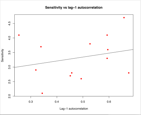
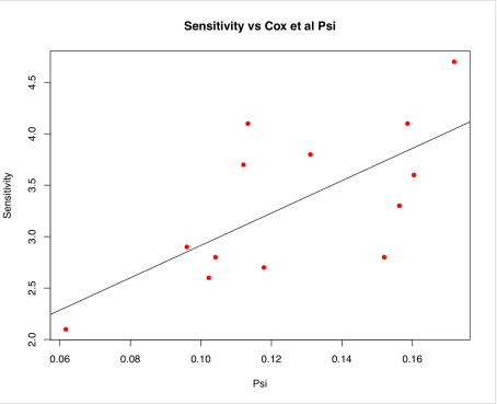
posted an article arguing that Cox et al underestimated their uncertainties. Unfortunately, he does this via an analysis of his own work that certainly does underestimate uncertainties, but which does not (I believe) accurately represent the Cox et al work. Here’s the Cox et al figure again, and below it another regression analysis of different data from Schneider’s blog.
Screenshot 2018-01-18 10.17.32
Screenshot 2018-01-25 10.45.40
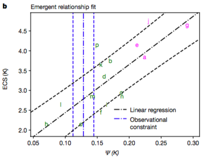
It’s clear at a glance that the uncertainty bounds on the Cox et al regression basically include most of the models whereas the uncertainty bounds of Schneider exclude the vast majority of his (I’m talking about the black dashed lines in both plots). I think the simple error here is that Schneider is considering only the uncertainty on the regression line itself whereas Cox is considering the predictive uncertainty of the regression relationship. The theoretical basis for most of the emergent constraint work is that reality can be considered to be "like" one of the models in the sense of satisfying the regression relationship that the models exhibit, ie it follows on naturally from the statistically indistinguishable paradigm for ensemble interpretation (I don’t preclude the possibility that there may be other ways to justify it). The intuitive idea is that reality is just like another model for which we can observe the variable on the x-axis (albeit typically with some non-negligible uncertainty) and want to predict the corresponding variable on the y-axis. So the location of reality along the x-axis is constrained by our observations of the climate system, and it is likely to be a similar distance from the regression line as the models themselves are.

Schneider then compares his interpretation of the emergent constraint method with model weighting, this being a fairly standard Bayesian approach. We also did this in our LGM paper, though we did the regression method properly so the differences were less marked. I always meant to go back and explore the ideas underlying the two approaches in more detail, but I believe that the main practical difference is that the Bayesian weighting approach is using the models themselves as a prior whereas the regression is implicitly using a uniform prior on the unknown. The regression has the ability to extrapolate beyond the model range and also can be used more readily when there is a very small number of models, as is typically the case in paleo research.

Here’s our own example from the paper which attempts to use tropical temperature at the Last Glacial Maximum as a constraint on the equilibrium sensitivity.
Screenshot 2018-01-25 11.01.56
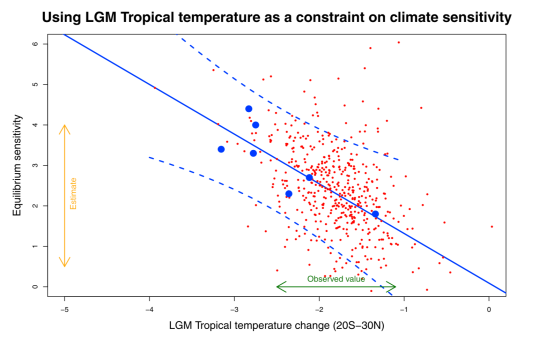
The models are the big blue dots (yes, only 7 of them, hence the large uncertainty in the regression). I used the random sampling (red dots) to generate the pdf for sensitivity, by first sampling from the pdf for tropical temperature and then for each dot sampling from the regression prediction. The broad scatter of the red dots is due to using t-distributions which I think is necessary due to the small number of models involved (eg even the uncertainty on the tropical temp constraint is a t-distribution as it was estimated by a leave-one-out cross validation process). But this is perhaps a bit of a fine detail on the overall picture. It is often not clear exactly how other authors have approached this and to be fair it probably matters less when considering modern constraints when data are generally more precise and ensemble sizes are rather larger.

We also did the Bayesian model weighting in this paper, but with only 7 models the result is a bit unsatisfactory. However the main reason we didn’t like it for that work is that by using the models as a prior, it already constrains the sensitivity substantially! Whereas if the observations of LGM cooling had been outside the model range, the regression would have been able to extrapolate as necessary.
Screenshot 2018-01-25 15.06.47
Here’s the weighting approach applied to the same question, with the blue dots marking the models, the green curve is the prior pdf (equal weighting on the models) and the thick red is the posterior which is the weighted sum of the thinner red curves. Each model has to be dressed up in a rather fat gaussian kernel (standard techniques exist to choose an appropriate width) to make an acceptably smooth shape. It’s different from the regression-based answer, but not radically so, and the difference can for the most part be attributed to the different prior.

Having said all that, I’m not uncritically a fan of the Cox et al work and result, a point that I’ll address in a subsequent post. But I thought I should point out that at least these two criticisms of Schneider and Benestad seem basically unfounded and unfair.

Thursday, January 18, 2018

More sensitivity stuff

After what feels like a very long hiatus, it seems that people are writing interesting stuff about climate sensitivity again. Just last week on Twitter I saw Andrew Dessler tweeting about his most recent manuscript which is up on ACP(D) for comment. My eyebrow was slightly raised at the range of values he found when analysing outputs of the MPI ensemble, 2.1 to 3.9K, until I realised that these were the outliers from their 100-member ensemble and eyeballing the histogram suggests the standard error on individual estimates (which I didn't see quoted) is around 0.5C or lower. Worth considering, but not a show-stopper in the context of other uncertainties we have to deal with. It would, I think, be interesting to consider whether more precise estimates can be calculated with a more comprehensive use of the data, such as by fitting a simple model to the time series rather than just using the difference between two snapshots. Which, coincidentally (or not) is something I might have more to talk about in the not too distant future.

Then just today, a new paper using interannual variability as an emergent constraint. By chance I bumped into one of the authors last week in Leeds so had a good idea what was coming but have not had time to consider in much detail. (The nature paper is paywalled but sci-hub.hk has a copy already.) Here's a screenshot of the main analysis for those who can't be bothered downloading it. The x-axis is a measure of interannual variability over the observational period, and the letters are CMIP models.


Using interannual variability to diagnose the equilibrium response has a somewhat chequered history, eg here and here for my previous posts though the links to the underlying papers are dead now so I've put the new ones here:


The central problem with the Schwartz approach is the strong (and wrong) assumption that the climate system has a single dominant time scale. It is easy to show (I may return to this in a future post) that the short time scale response simply cannot in principle directly constrain the equilibrium response of a two-time scale system. So this may be why the idea has not been followed up all that much (though in fact Andrew Dessler has done some work on this, such as this paper for example).

The latest paper gets round this by essentially using climate models to provide the link between interannual variability and equilibrium response. It remains possible that the models all get this wrong in a similar manner and thus the real climate system lies outside of their prediction, but this “unknown unknown” issue intrinsically applies to just about everything we ever do and isn't a specific criticism of this paper. My instinct is their result is probably over-optimistic and future work will find more uncertainties than they have presented, but that could just be a reflexive bias on my part. For example, it is not clear from what is written that they have accounted for observational uncertainty in their constraint, which (if they have not done) will probably bias the estimate low as uncorrelated errors will reduce their estimate of the real system's autocorrelation relative to the models where obs are perfect. There is also a hint of p-hacking in the analysis but they have done some quite careful investigation and justification of their choices. It will certainly provide an interesting avenue for more research.